\[\def\dif{\text{d}}\]

EoMs for Rotation \(\def\dif{\text{d}}\)

Newton’s second law relates mass to acceleration, and it is apparent that mass may be considered as a body’s tendency to resist a change in velocity. The analogue for rotation is moment of inertia. In a Newtonian framework, it is assumed that our aircraft is rigid and may be represented by a point mass, at the aircraft Centre of Gravity. In order to develop a Newtonian relationship for rotation, a means to represent the aircraft’s mass distribution is required, and how the mass distribution affects its tendency to resist rotational motion.

Newton’s second law (NII herein) can further be defined as the rate of change of inertia is equivalent to the applied force.

NII can be defined for rotational motion as the angular acceleration is proportional to the net torque and inversely proportional to the moment of inertia. angular momentum is defined as:

(29)\[\vec{H} = \vec{r} \times \left( m\vec{V}\right)\]

to define NII for angular motion, and determine the relationship between angular body rates and applied moments:

\[\left.\frac{d\vec{H}}{dt}\right|_{abs}=\vec{M}\]

\[\def\ii{\hat{\boldsymbol{\imath}}}\]

\[\def\jj{\hat{\boldsymbol{\jmath}}}\]

\[\def\kk{\hat{\boldsymbol{k}}}\]

Determination of angular momentum vector

The left hand side is will be built up by describing the aircraft as a system of discrete point masses - these are defined at positions \(\vec{r}_{\dif m}\) in aircraft body axes.

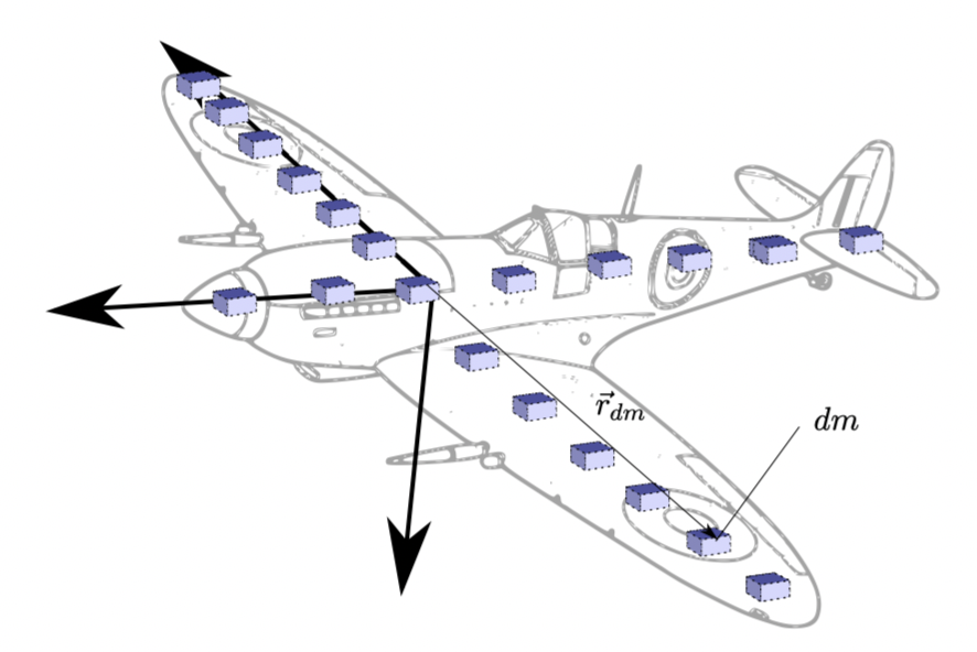
Fig. 54 Aircraft represented as point masses

\(\def\dif{\text{d}}\) For an elemental mass, \(\dif m\), located at \(\vec{r}_{\dif m}\), we perform the following steps to build our equations of motion:

1. Determine an expression for the translational velocity of \(\dif m\) due to aircraft rotation about the axis origin (aircraft centre of gravity), taking into account relative motion.

2. From this, develop an expression for the linear momentum of \(\dif m\)

3. Use Eq. (29) to develop an expression for the elemental angular momentum, given the linear momentum from the previous step.

4. Integrate the elemental masses over the entire aircraft to determine the angular momentum of the entire aircraft

5. Take into account the rate of change of angular momentum with respect to the inertially-fixed reference frame

Step 1 - Determine absolute velocity of \(\dif m\) with \(\vec{\omega}\neq0\)

Consider an elemental mass of the aircraft, \(\dif m\), at radius \(\vec{r}_{\dif m}\) - the velocity vector of this in body axes is simply the time rate of change of the position vector,

\[\left.\frac{d\vec{r}_{\dif m}}{dt}\right|_{Oxyz}\]

In flight mechanics the aircraft is assumed to be rigid5 so:

\[\left.\frac{d\vec{r}_{\dif m}}{dt}\right|_{Oxyz}=0\]

Just as for translation, the absolute velocity vector is required. Absolute velocity comprises components due to the velocity as defined in body axes, and also apparent velocity due to the time rate of change of the rotation vector, \(\vec{\omega}\).

As before, the Coriolis identities are integral to this process:

\[\begin{split}\begin{gathered} \left.\frac{d\ddagger}{dt} \right|_{abs} = \left.\frac{d\ddagger}{dt} \right|_{Oxyz} + \vec{\omega}\times\ddagger\\ \left.\frac{d^2\ddagger}{dt^2} \right|_{abs} = \left.\frac{d^2\ddagger}{dt^2}\right|_{Oxyz} + \dot{\vec{\omega}} \times\ddagger + 2\cdot\vec{\omega}\times\left.\frac{d\ddagger}{dt}\right|_{Oxyz}+\vec{\omega}\times\left(\vec{\omega}\times\ddagger\right)\end{gathered}\end{split}\]

To determine the absolute velocity we the first order identity:

\[\begin{split}\begin{aligned} V_{\dif m} = \left.\frac{d\vec{r}_{\dif m}}{dt} \right|_{abs} &= {\left.\frac{d\vec{r}_{\dif m}}{dt} \right|_{Oxyz}} + \vec{\omega}\times\vec{r}_{\dif m} \\ &= \vec{\omega}\times\vec{r}_{\dif m}\\ &=\left|\begin{matrix}\ii & \jj & \kk \\P & Q & R \\ x_{\dif m} & y_{\dif m} & z_{\dif m}\end{matrix}\right|\\ &= \begin{matrix} Q\cdot z_{\dif m} - R\cdot y_{\dif m}\\R\cdot x_{\dif m} - R\cdot z_{\dif m}\\P\cdot y_{\dif m}-Q\cdot x_{\dif m}\end{matrix}\label{eq:Step1}\end{aligned}\end{split}\]

Hence we have an expression for the absolute velocity of elemental mass, \(\dif m\).

Step 2 - Determine the linear momentum of \(\dif m\)

Normally, linear momentum has symbol \(P\), but this will cause issues with the term for roll rate, so \(\dif m\vec{V}\) will be used to represent the linear momentum:

\[\begin{split}\begin{aligned} \dif m\vec{V}_{\dif m}= \dif m\cdot\begin{bmatrix} Q\cdot z_{\dif m} - R\cdot y_{\dif m}\\R\cdot x_{\dif m} - P\cdot z_{\dif m}\\P\cdot y_{\dif m}-Q\cdot x_{\dif m}\end{bmatrix} \end{aligned}\end{split}\]

Note that the components of linear momentum in each axis consist solely of cross-coupling with terms from the other axes - if you get to this point, and you have direct terms in any row, then you have messed up one of your cross products.

Step 3 - Determine the angular momentum, \(\dif \vec{H}_{\dif m}\)

Using Equation (29), the angular momentum may be determined:

\[\begin{split}\begin{aligned} \dif \vec{H}_{\dif m}&=\vec{r}_{\dif m}\times \dif m\vec{V}_{\dif m}\\ &=\dif m\begin{vmatrix} \ii & \jj & \kk \\ x_{\dif m} & y_{\dif m} & z_{\dif m} \\ \left(Q\cdot z_{\dif m} - R\cdot y_{\dif m}\right) & \left(R\cdot x_{\dif m} -P\cdot z_{\dif m}\right) & \left(P\cdot y_{\dif m}-Q\cdot x_{\dif m}\right)\end{vmatrix}\\ &=\dif m \begin{bmatrix} P\left(y_{\dif m}^2 + z_{\dif m}^2\right) - Q\cdot x_{\dif m}\cdot y_{\dif m} - R\cdot x_{\dif m}\cdot z_{\dif m} \\ Q\left(x_{\dif m}^2 + z_{\dif m}^2\right) - R\cdot y_{\dif m}\cdot z_{\dif m} - P\cdot x_{\dif m}\cdot y_{\dif m} \\ R\left(x_{\dif m}^2 + y_{\dif m}^2\right) - P\cdot x_{\dif m}\cdot z_{\dif m} - Q\cdot y_{\dif m}\cdot z_{\dif m}\end{bmatrix}\end{aligned}\end{split}\]

Step 4 - Integrate over the entire aircraft

\[H= \int \dif H \dif m\]

(30)\[\begin{split}\begin{aligned} &=\begin{matrix} p\int\left(y_{\dif m}^2 + z_{\dif m}^2\right)\dif m - Q\int x_{\dif m}\cdot y_{\dif m}\dif m - R\int x_{\dif m}\cdot z_{\dif m}\dif m \\ q\int\left(x_{\dif m}^2 + z_{\dif m}^2\right) \dif m- R\int y_{\dif m}\cdot z_{\dif m}\dif m - P\int x_{\dif m}\cdot y_{\dif m}\dif m \\ r\int\left(x_{\dif m}^2 + y_{\dif m}^2\right) \dif m- P\int x_{\dif m}\cdot z_{\dif m}\dif m - Q\int y_{\dif m}\cdot z_{\dif m}\dif m \end{matrix}\end{aligned}\end{split}\]

The integral operators above are well-defined and standard quantities, called moments of inertia and products of inertia. The moments of inertia are:

\[\begin{split}\begin{aligned} I_{xx} = \int\left(y_{\dif m}^2 + z_{\dif m}^2\right)\dif m\\ I_{yy} = \int\left(x_{\dif m}^2 + z_{\dif m}^2\right)\dif m\\ I_{zz} = \int\left(x_{\dif m}^2 + y_{\dif m}^2\right)\dif m\end{aligned}\end{split}\]

The moments of inertia are always positive, and refer to a body’s tendency to resist motion about a given axis - and is a function of the mass distribution in a plane normal to that axis.

The products of inertia are: \(\def\itensor{\begin{bmatrix}I\end{bmatrix}}\) $\(\begin{aligned} I_{xy} = I_{yx} = \int x_{\dif m}\cdot y_{\dif m}\dif m\\ I_{xz} = I_{zx} = \int x_{\dif m}\cdot z_{\dif m}\dif m\\ I_{yz} = I_{zy} =\int y_{\dif m}\cdot z_{\dif m}\dif m\end{aligned}\)$

Products of inertia can be positive or negative, and are a little less intuitive to interpret, physically. They correspond to the net torque required to rotate at a constant rate about a given axis, and gives a measure of the degree of asymmetry of a body. An axisymmetric body (a well-balanced car tyre) has zero product of inertia about the axis of rotation, which results in a smoother ride - no net torque produced under constant rotation, and no net force at any instant. Conversely, if a car tyre is poorly-balanced, then there is a non-zero product of inertia, and a bumpier ride, and a non-zero net torque/force normal to the rotation axis.

We can substitute these into Equation (30) to get:

\[\begin{split}\begin{aligned} \vec{H}=\begin{matrix} H_x\\H_y\\H_z\end{matrix}&=\begin{matrix} P\cdot I_{xx} - Q\cdot I_{xy} - R\cdot I_{xz} \\ Q\cdot I_{yy} - R\cdot I_{yz} - P\cdot I_{xy} \\ R\cdot I_{zz} - P\cdot I_{xz} - Q\cdot I_{yz} \end{matrix}\\ &=\begin{bmatrix} I_{xx} & -I_{xy} & -I_{xz} \\ -I_{yx} & I_{yy} & -I_{yz}\\ -I_{zx} & -I_{zy} & I_{zz}\end{bmatrix}\begin{bmatrix}P\\Q\\R\end{bmatrix}\end{aligned}\end{split}\]

(31)\[\begin{aligned} &= \itensor\vec{\omega}\end{aligned}\]

where \(\itensor\) is the inertia tensor.

Simplification of the Inertia Tensor via symmetry

In general, most aircraft are symmetric about a longitudinal/vertical plane (slice it down the middle), and will also tend to have the principal yaw tensor axis aligned with \(z_b\). This means we can assume that: $\(I_{xy}=I_{yx}=I_{yz}=I_{zy}=0\)$

thus the equation for angular momentum is simplified to: $\(\begin{aligned} \vec{H}&=\begin{bmatrix} I_{xx} & 0 & -I_{xz} \\ 0 & I_{yy} & 0\\ -I_{zx} & 0 & I_{zz}\end{bmatrix}\begin{bmatrix}P\\Q\\R\end{bmatrix}\\ &= \itensor\vec{\omega}\\ \begin{bmatrix} H_x \\ H_y \\ H_z \end{bmatrix} &= \begin{bmatrix} I_{xx}\cdot P - I_{xz}\cdot R \\ I_{yy}\cdot Q \\ -I_{xz}\cdot P + I_{zz}\cdot R \end{bmatrix} \end{aligned}\)$

Step 5 - Determine the absolute rate of change of angular momentum

Again, using Equation (25) to determine the absolute rate of change of angular momentum:

\[\begin{split}\begin{aligned} \frac{\dif\vec{H}}{\dif t}_{abs}&=\frac{\dif\vec{H}}{\dif t}_{Oxyz} + \vec{\omega}\times\vec{H}_{Oxyz}\\ &=\frac{\dif\itensor\vec{\omega}}{\dif t}_{Oxyz} + \vec{\omega}\times\left(\itensor\vec{\omega}\right)\\ &=\frac{\dif\itensor}{\dif t}\vec{\omega}+\itensor\frac{\dif\vec{\omega}}{\dif t} + \begin{vmatrix} \ii & \jj & \kk \\ P & Q & R \\ \left(I_{xx}\cdot P - I_{xz}\cdot R\right) & \left(I_{yy}\cdot Q\right) & \left(-I_{xz}\cdot P + I_{zz}\cdot R \right) \end{vmatrix}\end{aligned}\end{split}\]

since the rigid aircraft assumption has already been invoked, the products and moments of inertia are constant in time, hence the time rate of change of \(\itensor\) cancels to zero

\[\begin{split}\begin{aligned} &={\frac{\dif\itensor}{\dif t}}\cdot\vec{\omega}+{\frac{\dif\vec{\omega}}{\dif t}\cdot\itensor} \hspace{1cm}+ \begin{vmatrix} \ii & \jj & \kk \\ P & Q & R \\ \left(I_{xx}\cdot P - I_{xz}\cdot R\right)& \left(I_{yy}\cdot Q\right) & \left(-I_{xz}\cdot P + I_{zz}\cdot R \right) \end{vmatrix}\\ &= \begin{bmatrix}I_{xx}\cdot\dot{P} - I_{xz}\cdot\dot{R}\\I_{yy}\cdot\dot{Q}\\I_{zz}\cdot\dot{r} - I_{xz}\cdot\dot{P}\end{bmatrix} + \begin{bmatrix} Q\left(I_{zz}\cdot R - I_{xz}\cdot P\right) - R\left(I_{yy}\cdot Q\right) \\ R\left(I_{xx}\cdot P - I_{xz}\cdot R \right) - P\left(I_{zz}\cdot R - I_{xx}\cdot P \right) \\ P\left(I_{yy}\cdot Q\right) - Q\left(I_{xx}\cdot P - I_{xz}\cdot R\right)\end{bmatrix}\end{aligned}\end{split}\]

collecting terms of the moments and products of inertia yields

\[\begin{split}\begin{aligned}\begin{bmatrix} \dot{H}_x\\ \dot{H}_y\\ \dot{H}_z\end{bmatrix}_{abs} &= \left[\color{blue}{\begin{matrix} \dot{P}\cdot I_{xx} \\ \dot{Q}\cdot I_{yy} \\\dot{R}\cdot I_{zz}\end{matrix}} \hspace{.5cm} \begin{matrix} + \\+\\+\end{matrix} \hspace{.5cm} \color{red}{\begin{matrix} Q\cdot R\left(I_{zz} - I_{yy}\right) \\ P\cdot R\left(I_{xx} - I_{zz}\right) \\ P\cdot Q\left(I_{yy} - I_{xx}\right)\end{matrix}} \hspace{.5cm} \begin{matrix} - \\+\\+\end{matrix} \hspace{.5cm} \color{green}{\begin{matrix}\left(\dot{R} + P\cdot Q\right) I_{xz} \\ \left(P^2 - R^2\right) I_{xz} \\ \left(Q\cdot R - \dot{P}\right) I_{xz}\end{matrix}} \right]\end{aligned}\end{split}\]

where:

• \(\color{blue}{\text{Blue terms}}\) represent a change to angular momentum due to a change in angular rate about that axis.

• \(\color{red}{\text{Red terms}}\) terms represent gyroscopic precession, which causes an increase in angular momentum about an axis due to the product of angular rates about other axes, and the respective differences in their moments of inertia.

• \(\color{green}{\text{Green terms}}\) terms represent an increase to angular momentum cross-coupling (due to the off-diagonal terms of the inertia matrix), wh ich is caused by a combination of angular acceleration around a coupled axis, and the product of combination of angular rates about two other axes. It should be appreciated that if we did not simplify the inertia matrix, the number of green terms would be much larger.

Thus the rotational equations of motion have been derived, and the right hand side is the non-conservative moments which is the moments applied to the airframe.

(32)\[\begin{split}\left[{\begin{matrix} \dot{P}\cdot I_{xx} \\ \dot{Q}\cdot I_{yy} \\\dot{R}\cdot I_{zz}\end{matrix}} \hspace{.5cm} \begin{matrix} + \\+\\+\end{matrix} \hspace{.5cm} {\begin{matrix} Q\cdot R\left(I_{zz} - I_{yy}\right) \\ P\cdot R\left(I_{xx} - I_{zz}\right) \\ P\cdot Q\left(I_{yy} - I_{xx}\right)\end{matrix}} \hspace{.5cm} \begin{matrix} - \\+\\+\end{matrix} \hspace{.5cm} {\begin{matrix}\left(\dot{R} + P\cdot Q\right) I_{xz} \\ \left(P^2 - R^2\right) I_{xz} \\ \left(Q\cdot R - \dot{P}\right) I_{xz}\end{matrix}} \right] = \begin{bmatrix} L \\ M \\ N\end{bmatrix}\end{split}\]

---

5

The study of flexible aircraft is called aeroelasticity, and is easier to explore with a Lagrangian approach, as opposed to the Newtonian approach of this course. Hopefully more on that to come at IIT.